This is my quarterly missive intended primarily for my fellow financial professionals wherein I share items I have run across or thought about this quarter which I think might be beneficial to you. Enjoy!

For the rest of 2018 I have seminars for CPAs scheduled (through Surgent) in Texas (Dallas and Fort Worth), Georgia (Atlanta twice and Duluth), and North Carolina (Greensboro, Charlotte, and Morrisville). More will be added soon.

I would love to see you at one of those sessions, and if you are looking for a speaker at your professional conference or event, please feel free to contact me for more information.

First, there is a very human tendency to “do something” – even when the best thing to do would be nothing. The problem compounds when you can increase your income by doing something, and the customer really wants you to do something, even if it is not particularly helpful. You may think I’m talking about active investment management, but I’m not (well, I’m not only talking about that). Medicine has the same problem, and of course it’s easier to see the mote in another’s eye. (Politics has the same problem too.)

“Evidence-based” medicine (and investing) is the right answer, but it is very, very hard to do.

Second, I emailed my consulting clients about this last August, and put it in this newsletter in October. Bloomberg noticed it in January: Land Is Underrated as a Source of Wealth. Be sure to note the caveats I made in the earlier piece.

Third, I emailed this link to my consulting clients on January third with the subject line “Optimistic Economists Make Me Nervous.” You know how the market has done since then.

Fourth, I wrote a long paper on being a financial professional a long time ago (here), but a good perspective from John Bogle is summarized here, as follows:

1. Places the interests of clients in particular and the welfare of society in general above its own.

2. Has a specialized body of knowledge and a specialized code of conduct that sets out professional skills, practices, and performances unique to the profession. Taken together, these develop the capacity to render judgments with integrity under conditions of ethical uncertainty.

3. Defines an organized approach to learning from experience, both individually and collectively.

4. Participates in a professional community that monitors and oversees the behavior and competencies of its members.

Fifth, as I have noted many times, humans are captivated by stories, but largely oblivious to data. The NYT had a good column on how bad we are at this. It applies to investing obviously – we really want certainty and conclusions but all that is available is uncertainty and probabilities

When a client asks you what you think the market will do this year, how have you answered? I think there are two reasonable answers based on history:

1. Most likely between a 29% loss and a 53% gain, but there is about a 1-in-20 chance it could be outside that range. (The average 12-month return from 1926-2016 for U.S. stocks was 11.94% with a standard deviation of 21.09%. 95% would be within 1.96 standard deviations so 11.94% +/- 41.34% is a range of -29.40% to +53.28%.)

2. Most likely between a 21% loss and a 45% gain, but there is about a 1-in-20 chance it could be outside that range. (If you assume that the world is safer or different now so post-WWII numbers are a better estimate of the future, the average 12-month return from 1946-2016 for U.S. stocks was 12.22% with a standard deviation of 16.77%. 95% would be within 1.96 standard deviations so 12.22% +/- 32.87% is a range of -20.65% to +45.09%.

You could also argue that equity returns will be lower by some amount – maybe 1% lower because of lower inflation and another 2-3% lower from a lower ERP going forward so the whole distribution is shifted down by that amount. If so you can adjust the ranges down by 3-4%. I also do think that starting post-WWII is too aggressive, but I can understand the logic of someone using it and I wouldn’t say they are wrong. I would point out though, if that is the correct distribution then 2008 was a huge outlier. If we use from 1926 it was fairly normal. (The worst 12-months in that debacle was March 2008 to February 2009, which had a 42.48% loss – a rare but reasonable 2.53 standard deviation event if we use from 1926 to the month prior to that period, but an improbable 3.26 standard deviations if we start in 1946.) So, my best answer would be: “Most likely between a 33% loss and a 50% gain, but there is about a 1-in-20 chance it could be outside that range.”

Also, if you want to know the 100-year-flood number that would be 2.58 standard deviations. 11.94% minus a 3.5% adjustment for lower returns in the future is 8.44% minus 2.58*21.09% = -45.89%. (Of course, there is also a 1-in-100 chance of a positive 62.77%) Keep in mind, the worst-case scenario that has ever happened (in any area, not just market returns) was not the worst-case just prior to it happening. Think about that for a while.

I am anticipating some questions, here are the answers:

1. You undoubtedly think those answers are wrong – you just really don’t think the range is that high. I feel the same way, but I know I’m wrong…

2. Clients would be profoundly unhappy with an answer like that. I know, but it is what it is. If I could improve on those figures I would be running a hedge fund engaged in market timing.

3. I used the CRSP 1-10 figures, not the S&P 500 because the question is “what do you think the market will do?” not “what do you think the S&P 500 will do?” Most people think it is the same thing, and substantially they really are, the correlation is 99.09%, the difference in annual returns have averaged 26 basis points (advantage S&P500) and average difference in standard deviation was 25 basis points (advantage CRSP 1-10). So, I wouldn’t really quibble if someone used the S&P500 to do these calculations, but I didn’t.

4. I didn’t have 2017 year-end figures when I computed this, so that’s why I used through 2016 throughout. Any differences will be trivial, one year just doesn’t have that much weight.

5. I rounded off to a reasonable number of decimal places as I typed this up, but all the calculations used all the decimal points I had available – just in case you are following my math and find something slightly off.

6. The correct returns to use for this exercise are arithmetic, not geometric. If you want to convert, the rough estimate (but it’s pretty good) is given by squaring the standard deviation (to get the variance), then subtracting half of that from the return. For example, I said, “The average 12-month return from 1926-2016 for U.S. stocks was 11.94% with a standard deviation of 21.09%” 0.2109^2= 0.0445 That divided by 2 equals 0.0222. 11.94% minus 2.22% is 9.72% geometric return, which is the figure you are more accustomed to seeing. For more on this topic you can see my calculator here.

7. I used 12-month periods, the maximum drawdown to expect is higher because it can go on for longer than 12-months. For example, from October 2007 through February 2009 was a 50.19% decline, but 2008 was just 36.71%, and as mentioned above, March 2008 to February 2009 had a 42.48% loss.

8. I used a normal distribution rather than a log-normal one because for a one-year period they are trivially different. There was already more than enough math here to make most people’s heads hurt without introducing that complication.

Sixth, good article on investing in commodities here. Not new info. I sent the papers referred to out years ago to our consulting clients. I also sent this (registration required, unfortunately) way back in 2015.

Seventh, in the January client newsletter (not this one) I talked about some tax strategies given the new law, but there are more items that are just … odd. Here are a few that occur to me:

1. Usually single dollar thresholds are half of married, but the $10k SALT deduction and $750k mortgage limits are the same for each. That means most single people, if they own a home, will still itemize, but most married people won’t. Assume married couple with one spouse making $150,000 and one making $50,000. AGI is thus $200,000 and they own a home with a $400,000 mortgage at 4% ($16,000 annual interest). State income taxes are $10,000. Real estate taxes are another $5,000. Married, their itemized deductions are $16k (mortgage interest) + $10k (limit on SALT) = $26k. That is slightly over the $24k standard deduction. But if they don’t get married, suppose the state taxes are $7,500 and $2,500 (I just pro-rated based on the income) on the respective spouses. If they have the lower paid spouse take the standard deduction of $12k, then the deduction for the higher paid spouse is the same $26k it was before for a total of $48k of deductions. Also, if there is a home (or two) with a $1,500,000 mortgage (in both names, or one in each), don’t get married (if both have taxable income of at least a moderate amount).

2. The thresholds mentioned in the previous point aren’t adjusted for inflation, but the standard deduction is, so as time goes by fewer and fewer people will itemize.

3. If interest rates go up, more people will itemize because the mortgage interest deduction is limited by the principal balance not the interest paid. This also means that poor credit risks are more subsidized by the tax code than good credit risks (just as it is now). But as mentioned in the previous point, if rates have increased because of inflation, the effect will be offset somewhat.

4. Alimony agreements entered into after 2018 will no longer be tax deductible to the payor (nor taxable to the recipient). This eliminates tax arbitrage (since the marginal bracket of the payor is usually higher than the payee). However, there is a way to get some of it back. Assume husband and wife have a mortgage on their home which both parties are responsible for (like normal with a couple). Assume the husband is the alimony payor. After divorce, if they agree that he is responsible for the mortgage the interest is still deductible to him. And, since his filing status is now single, he will actually get the deduction. The couple in the previous example (#1) divorces and the higher paid spouse takes the mortgage obligation and taxes as part of the settlement That spouse’s itemized deductions are still $26,000 even though the standard deduction (single) would have been just $12,000. Now some of each payment would have been principal on the mortgage – so perhaps a refi into the longest-term interest only mortgage available would be appropriate.

5. The marriage penalty is much larger than it was previously.

6. In Georgia it makes a great deal of sense to do the education tax credit or the rural hospital tax credit (or, most likely, both) to get to the standard deduction threshold. Assume AGI of $250,000 (MFJ) and they own a home with a $350,000 mortgage at 4% ($14,000 annual interest). State income taxes are $15,000. Real estate taxes are another $5,000. Their itemized deductions are thus $24,000 and the mortgage deduction was useless since they could get $24,000 from taking the standard deduction. But if the couple makes a $11,111 contribution to a rural hospital they get $10,000 back on state taxes. They get a $11,111 charitable deduction on their federal return, combined with $10,000 SALT means they are at $21,000 of deductions without the mortgage. So, they “lose” $1,111 to get an increase of $11,111 in deductions that is worth (at 24% bracket) $2,667. ($5,000 state income taxes, + $5,000 property taxes + $11,111 of charitable deductions + $14,000 of mortgage interest = $35,111)

7. It may make sense to itemize federally even if slightly under the standard deduction. In most states you can’t itemize for state taxes unless you itemize for federal. For example, in Georgia the state tax rate is 6% and the state standard deduction is just $3,000. The federal standard deduction is $24,000. Suppose our taxpayer is in the 24% marginal federal bracket. If the taxpayer has $23,000 of itemized deductions and itemizes it costs $1,000*0.24=$240 in federal taxes but saves ($23,000-$3,000)*0.06=$1,200 on state taxes. The breakeven in this case is $19,000. If itemized deductions are between $19,000 and $24,000 the taxpayer should itemize even though they are under the standard deduction.

8. If you are a business owner that qualifies for the pass-through deduction, be careful about giving ownership to employees. The deduction is limited to half of w-2 wages (if over the taxable income threshold). Partners do not receive w-2 income, regardless of how small the ownership percentage is. For example, suppose a (married) owner makes $300,000/year from the business and has one employee that makes $120,000. The pass-through deduction would be 50% of w-2 wages, up to 20% of the self-employment income. In this example (since I made it up) those are both $60,000. In the 24% tax bracket that is worth $14,400 of tax savings. If the employee is given any amount of ownership, that deduction is lost.

Eighth, a particularly stupid headline: The Top 25 Stocks Of 2017 Trounced The S&P 500

Now wouldn’t that be true every year (since there is always cross-sectional dispersion)? And wouldn’t the bottom 25 stocks always get trounced by the S&P 500.

This is like saying, “The tallest people in the world are taller than most people.” Um, ok.

Ninth, more stupidity. I was at a conference where about half of the speakers (maybe more) talked about where we are in the “business cycle” and how you should invest (or hedge) based on that – many have either had a slide that depicted it, or they made the graph with their hand in the air. It makes me crazy. I defy you to find actual data that depicts something resembling the graphs. Googling “business cycle graphs” will give hundreds of examples that look like this:

They are all bogus. Here is what the graph of the actual data looks like. Go take a look at that, I’ll wait.

Ok, you say, that isn’t fair, what they meant was change in real GDP from the prior period in which case the graph shouldn’t trend up (like most do) but it will show the changes from trend more clearly. That graph is here. Take a look at it.

It doesn’t look like a cycle to me, and it certainly doesn’t look like a sine wave like virtually every graph in every presentation and economics textbook. Furthermore, I defy you to take a portion of the graph and predict the next section to the right. In other words, predict where we are the “cycle” without cheating and looking at the corresponding dates (and in the graph you have the revised GDP data that you wouldn’t even have available in real time). And if you can’t tell where you are in the cycle (if there is one) what exactly would be the point of basing your investment strategy on it?

Tenth, I was in an investment committee meeting this quarter for one of our consulting clients and there was a representative from Blackrock there who usefully divided investment strategies into three buckets (my characterization and names of the groupings):

1. Indexed – market-cap weighted, almost free, “beta”
2. Factor-based – tilts to various factors identified in academia, rules-based, passive, cheap, “smart beta”
3. Active – “alpha” (excludes the returns that come from the previous two sources)

In our businesses we can invest in any of the three strategies – or a combination. Here are the pro’s and con’s:

1. Indexed – certain beta (you get the market, and there is no tracking error).
2. Factor-based – probable alpha (the factors are well-documented and persistent, but there can be long periods of underperformance).
3. Active – doubtful alpha.

There are three reasons I believe the active alpha is doubtful, and they build on each other:

1. Active alpha may not exist. After adjusting for factor exposures, it looks like active manager outperformance is random (i.e. luck, not skill).

2. If active alpha exists, I still have no way to identity the skillful manager in advance. The time period required to separate the signal from the noise is just too long – I have calculated that if a manager has outperformed his or her benchmark by 2% per year on average (a 2% alpha is, of course, huge), 56 years of data would be required to know with confidence he or she was actually better (not 2% better – just better at all) and that it wasn’t just luck (assumes 90% correlation and 20% standard deviation).

3. If active alpha exists, and if you can identify the manager who has the skill, that manager will rationally extract most (or maybe even more since the data is noisy) of the returns in fees (or what economists call “rents”). There is no rational reason for a manager not to extract the extra value for themselves. Economic rewards flow to the scarce factor of production, and in investing, capital is not the scarce factor, the ability (or, more cynically, the appearance of the ability) to generate alpha is.

Eleventh, I read this article on business management (or, more precisely, how not to be confused about what constitutes good management), and I'm including it here because the three points at the end apply perfectly to investment management as well:

1. Recognize the role of uncertainty
2. See the world through probabilities
3. Separate inputs from outcomes

Those three points are interrelated. I would put it this way: Because everything in the world is more or less uncertain, you should think in terms of probabilities and realize that good decisions sometimes lead to poor outcomes (and vice-versa). As I wrote a long time ago (and reposted a year ago here):

[A] good decision is not the same thing as a good outcome, though they should be correlated. For example, investing all of your retirement funds in lottery tickets or one single stock is a bad decision even if you happen to win the lottery or the stock skyrockets. Conversely, investing in the market (prudently, with an appropriate asset allocation, etc.) is a good decision even if the market subsequently crashes.

Twelfth, it looks like advisors are more ignorant than greedy. I’m not sure which is worse, but a fiduciary standard doesn’t fix stupid.

Specifically, even in their own portfolios, advisors engage in far too much:

1. Return Chasing
2. Active Management
3. Turnover
4. Under-Diversification
5. Use of High-Cost Investments

This leads to -3.07% alpha for clients and -3.00% for themselves (net of commissions received back on their own trades). Both figures were statistically significant.

Thirteenth, the more I think about investing, the more I think the key questions are epistemological – that the most crucial question is, “but how do we know?”

As WK Clifford concluded in his 1877 essay, The Ethics of Belief, “To sum up: it is wrong always, everywhere, and for anyone, to believe anything upon insufficient evidence.”

All too often “belief” comes via a free (wholesaler) lunch and a good story.

Fourteenth, the Credit Suisse Global Investment Returns Yearbook 2018 is out and available here.

Fifteenth, one of our consulting clients just asked a good question, “Which portfolio has the least amount of risk – 100% fixed income or something like a 20/80 portfolio.”

My response:

Great question.

100% fixed income absolutely isn’t the lowest risk. It greatly depends on the time period, assumptions, what duration bonds, etc. but here is the last 40 years (1978-2017), using CRSP 1-10 and five-year treasuries, rebalanced monthly:

		% Stocks
1978-2017	5yr TSY	5%	10%	15%	20%
CAGR	7.01%	7.31%	7.61%	7.90%	8.19%
Annualized Sigma	5.47%	5.29%	5.23%	5.29%	5.47%
Max Drawdown	8.89%	7.76%	6.67%	6.54%	6.60%

You would think that using (relatively) short-term treasuries they would be much safer than having any stocks at all, but they aren’t. Of course, I started (on purpose) after we went off the gold standard, so it reflects higher bond risk now than may have existed in the very early data. We use 20/80 as the most conservative portfolio for our clients. Notice that the standard deviation of that is the same as all bonds. So, it isn’t (from that perspective) riskier, and from a max drawdown perspective it is actually safer. But of course, the return has been much better.

Remember the MPT curve curls under on the left side if it is dawn all the way from 100% bonds to 100% stocks. Using the data from the table above, the “efficient frontier” technically only goes from the 10/90 to the 100/0 combinations (but it’s drawn wrong in lots of textbooks) – the bottom two dots (0/100 and 5/95) would be inefficient. Ballpark you could say that 90% bonds are safest, 100% bonds is the same risk as 80% bonds and 95% bonds is the same risk as 85% bonds.

Sixteenth, there is a topic on which I listen carefully to clients and then mostly ignore what they just told me…

Clients think that the fact that “Mom lived to be 98” or “the men in my family all die before 75” is relevant information for designing their financial plan. It isn’t. Socioeconomic class matters (largely because diet, exercise, and smoking are very correlated to class), but genetics don’t matter much at all. More evidence supporting that view just came out.

Seventeenth, I got into a discussion on the size premium recently. I thought I would share my thoughts and some updated data.

1. Small-cap does, on average, have higher returns than large-cap. This is good.
2. Small-cap also has, on average, higher risk than large-cap. This is bad.
3. Taking both of the previous points into account we find that small-cap does not have higher returns after adjusting for the risk.

In other words, levering a large-cap portfolio to small-cap risk levels would produce a higher return than buying small-cap. We can see this by looking at the monthly Sharpe ratios by CRSP Decile (1 is largest, 10 is smallest):

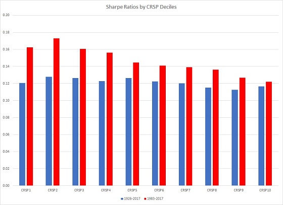
I showed the last 35 years as well as the full sample for two reasons:

1. Index data doesn’t have costs and the trading costs of small-cap would have been high in the early years. In other words, I’m not sure investors could have captured the full returns in the “old days.”

2. Rolf Banz published his landmark paper on the small-cap premium in 1981. It would be rational for it to have attenuated since then.

So, since small-cap doesn’t seem to “work” after taking the volatility into account, why do we (and others) own it? There are three reasons (the first is a somewhat cynical one and not the reason we own it):

1. Since most investors don’t risk-adjust their performance and since the returns are higher on small-cap, owning small-cap will make performance look better. (This is the same reason that high beta stocks seem to have lower returns – managers over-own them because they generally can’t use leverage and need to beat their benchmark).

2. The value-added by various factor exposures I think are larger in small-cap than in large-cap. Here is a ranking of the returns on various Russell indexes over the past 35 years (for consistency) to show how the value effect has manifest in different market caps:

As you can see, the value premium in large-cap (value minus growth) was just 97 bps vs. 355 in small-cap. In this particular data small value doesn’t appear to outperform large value, but I think that is just this dataset. The Russell 2000 index is a very poor one to invest in (due to front-running of the index reconstitutions). In other words, the spreads of value and growth within market cap I think are valid, but the large vs. small not.

3. There is a diversification benefit. Small value (R2000V) is the least correlated with large (R1000).

So, to recap, you want to own small because it improves diversification, but small growth is terrible, so owning small value is much better. Returns will be much better for the client, but not as much as you would think once risk is considered.

Eighteenth, Tenancy by the Entireties (TBE), if available, is an easy way to reduce risk for clients. If clients are in states that have it, and those clients are married, we should, as financial planners, make sure that is addressed. Of the 51 jurisdictions in the US (50 states plus DC):

• 9 are community property
• 42 are common law, of those
• 25 have TBE for real estate
• 18 of those have TBE for personal property as well
• 17 don’t have TBE

See this list (scroll down) to find out where it is available.

Nineteenth, many people will be “rich” (in income at least) at some point: “[M]ore than 10% of wage-earners will, at some point in their lives, be among the Top 1%! Perhaps more impressively, more than 50% of Americans will at some point be in the Top 10%.” (From this article.)

The original source is CNN and is presumably true – and not at all what people think when they are talking about those cohorts.

Twentieth, the producer of the show The Big Bang Theory groks investing now:

The stock market, as measured by the S&P 500 Index, has returned about 10% per year over the last 90 years, but there are very few individual years in which it has ever actually returned that amount. In fact, how many of those 90 years do you think the S&P 500 was up more than 20% or down more than 20% for that year? The answer is 40. Astounding, right? I wish somebody had explained that to me decades ago. Then I would have known to look at stock market returns in terms of decades—not years, months, days, or hours. I would understand that so many of those articles and cable news pieces are just noise, designed to keep an audience obsessed and unsettled.

Twenty-first, as humans we are very good at pattern recognition. Too good it turns out. We see patterns even in random data. For example, it seems obvious to people that in the stock market there are bull markets and bear markets, but what we call a bull market is just when the random series happened to be positive a few times. And a bear market is just when the random series happened to be negative a few times. This feels deeply and intuitively wrong (even to me), but it isn’t.

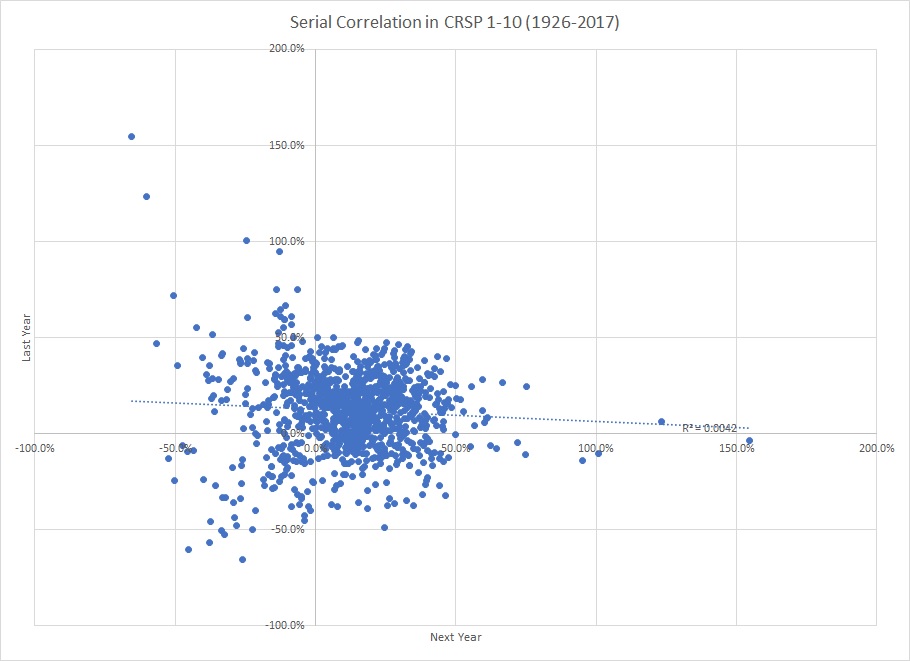
Here is a plot of all the rolling 12-month returns on the total stock market with the prior year returns on the y-axis and the subsequent year on the x-axis – do you see any pattern?

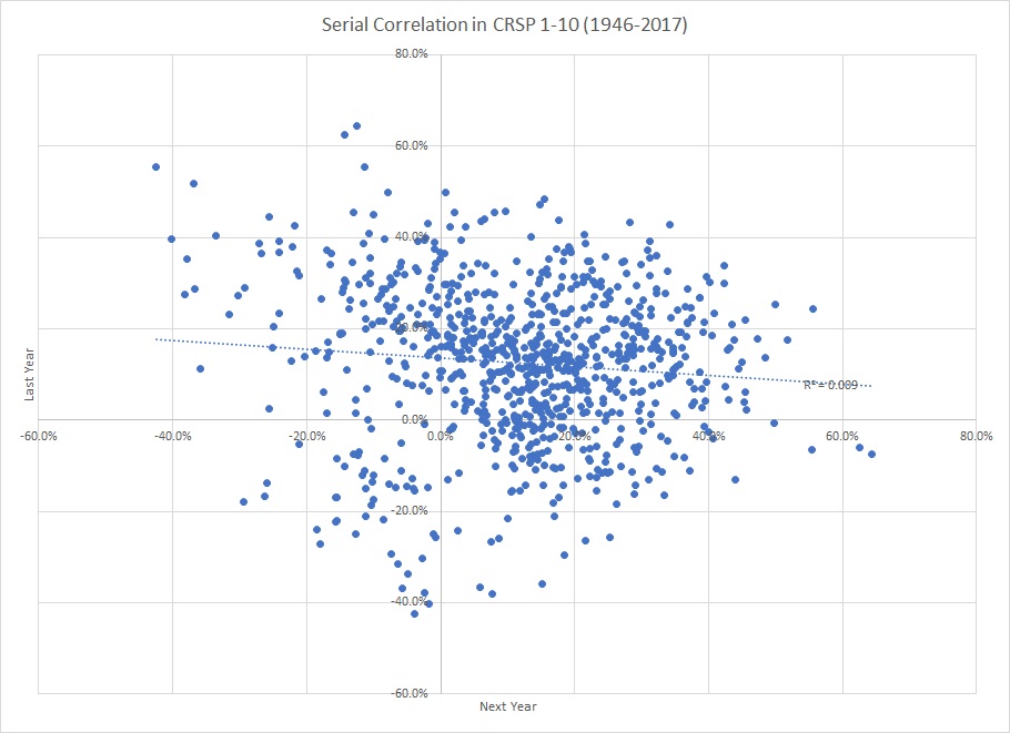
I don’t see one, the correlation is just -6.46% so obviously the R^2 is just 0.0042 (-0.0646 squared). There are some severe outliers on that graph from the early 1930s. What if we restricted the data to post-WWII?

The correlation is more negative, but still negligible, at -9.51% so the R^2 is still just 0.0090.

So, if all the prognosticators would stop referencing past returns when making their (mostly useless) predictions, that would be nice. History teaches us the 21.1% 2017 return doesn’t indicate anything meaningful about 2018.

Twenty-second, notwithstanding my previous point, and at the risk of data-mining/cherry-picking/whatever, I was thinking…

Let’s assume for a moment that the market does move in cycles and that each generation or so roughly replays the experience of the previous ones.

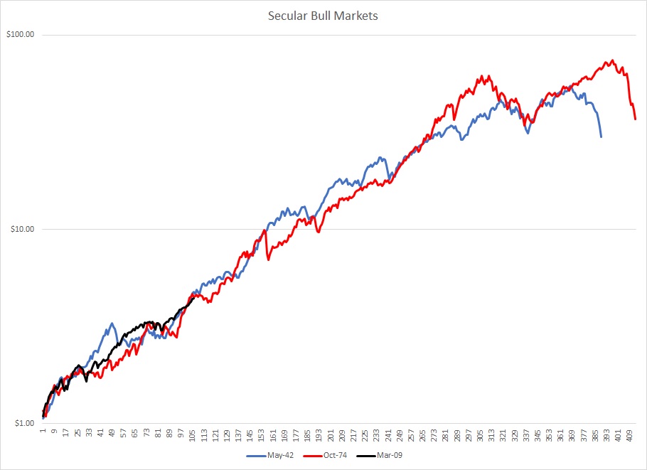
So, it occurred to me to align the last few cycles starting from the low points in 4/1942, 9/1974, and 2/2009 to see what might lie ahead. Here is a graph of the growth of $1 from each of those points:

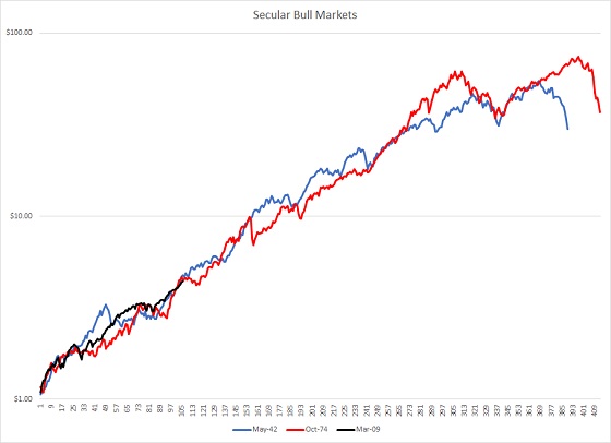
If this cycle is like the last two, we have 21½ to 23½ strong years ahead of us with average annual returns of over 12%!

Again, that is not a prediction, but I thought it was very interesting – particularly as “everyone” is talking about how old this bull market is and implying the good times must end soon. Obviously though, market valuations are very different now than at the equivalent time in the previous cycles because we didn’t go down nearly as far (the market didn’t get nearly as cheap in the GFC). We are nine years from the March 2009 low. In May 1951 and October 1983 (nine years into the previous cycles) the Shiller PE (aka CAPE) was 12 and 10 vs. the current 33.

Twenty-third, two spreadsheets that I created many years ago (and that I think are very cool, though the fact that I think a spreadsheet can be cool is probably indicative of my lack of coolness) have been updated with data through the end of 2017. Both allow you to easily see historical market context (in the US, which is a severe limitation). As with all my spreadsheets the yellow cells are the input cells. I encourage you to play with these and let me know if you like them.

The Historical Market Downturns spreadsheet lets you select a mix of stocks and bonds, the time period, and whether you want to see nominal or real results and shows the frequency and severity of downturns.

The 2nd and 3rd tabs on the Investment Return Matrix debunk what I think is a common misconception. The chart on the second tab shows that as your holding period lengthens (and you can change the investment mix and inflation adjustment on the top of the first tab) your average annual returns get less extreme. Most people leave it at that and think that their distribution of wealth sort of averages out over time if they hold on, but it certainly doesn’t! The third tab shows that even though the average annual returns smooth out, the ending values widen. Put another way, over a one-year time horizon, returns on a 60/40 portfolio adjusted for inflation have been as low as -23.4% and as high as 33.7%, while over 20 years the range has been just 0.8% to 10.0%. But a 9.2% difference, compounded over 20 years is an enormous amount of money! Over a one-year period the ratio of the most to the least you have is 1.75, over 20 years it was 5.70. Risk does not diminish over time, it increases. That is a 60/40 real portfolio! For all stocks in nominal dollars, the one-year range (again, the highest value divided by lowest value) is 2.77 while the 20-year range is 14.15! Again, I don’t believe that is how people understand it.

Twenty-fourth, I updated a spreadsheet with Russell data from 1979-2017. It lets you see the probability (using only this data, of course we have much more evidence elsewhere) that small beats large (just 29%) or value beats growth (45%), or small value beats small growth (74%).

Again, yellow cells at the top are the inputs. There are a few graphs on the tabs at the bottom that I think are interesting too.

Twenty-fifth, this spreadsheet shows we are pretty much on trend, but it is probably misleading – current valuations are above trend, historical returns are probably not the trend going forward. See Shiller’s PE and Tobin’s Q for example.

Finally, my recurring reminders:

J.P. Morgan’s updated Guide to the Markets for this quarter is out and filled with great data as usual.

Jonathan Clements, Morgan Housel, and Larry Swedroe, all continue to publish valuable wisdom. Just a reminder to go to those links and read whatever catches your fancy since last quarter.

That’s it for this quarter. I hope some of the above was beneficial.

Addendum:

If you are receiving this email directly from me, you are on my list of Financial Professionals who have requested I share things that may be of interest.  If you no longer wish to be on this list or have an associate who would like to be on the list, simply let me know.

We have clients nationwide; if you ever have an opportunity to send a potential client our way that would be greatly appreciated.  We also have been hired by some of our fellow advisors as consultants to help where we can with their businesses.  If you are interested in learning more about that arrangement, please let us know.

We also offer a monthly email newsletter, Financial Foundations, which is intended more for private clients and other non-financial-professionals who are interested.  If you would like to be on that list as well, you may edit your preferences here.

Finally, if you have a colleague who would like to subscribe to this list, they may do so from that link as well.

Regards,
David

Disclaimer: The information set forth herein has been obtained or derived from sources believed by author to be reliable. However, the author does not make any representation or warranty, express or implied, as to the information’s accuracy or completeness, nor does the author recommend that the attached information serve as the basis of any investment decision. This document has been provided to you solely for information purposes and does not constitute an offer or solicitation of an offer, or any advice or recommendation, to purchase any securities or other financial instruments, and may not be construed as such.